
Introduction
AWS DynamoDB (DDB) has proved to be one of the most robust, scalable and cost-effective NoSQL solutions out there. Unlike SQL table rows, data is stored as JSON objects called items. There are multiple ways you can store those items on your table(s). In other words, there are several design patterns for DDB:
- Multi-table design: Only one entity is stored in one table, similar to normalised RDBMS.
- Single-table design: Multiple entities are stored in a single table in a denormalized fashion.
- A mix of both: Multiple entities are stored in a single table where some entities are related to others from another table, which also contains one or more entities.
Which one to choose depends on your application and requirements. In this article, we will focus on the single-table design, where we will look at how our table can evolve depending on new access patterns.
Let’s get started.
Prerequisites
Not so fast! Before diving deep into the article, make sure you understand DDB fundamentals:
Example: Sensor Management
Overview
The example is based on a table called “sensor-management”, which stores information about IoT sensors and their locations. As mentioned, multiple entities are stored in the table according to the single-table design. Below, there is an image presenting how the entities are related to each other via the ER diagram:
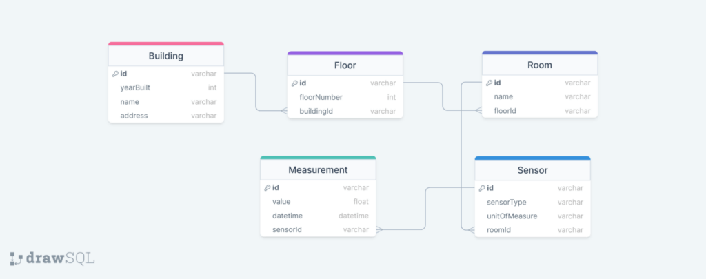
One building can have multiple floors; one floor can have multiple rooms; one room can have multiple sensors; one sensor can have multiple measurements. Basically, we have several one-to-many relationships between the entities.
We are interested in the following access patterns, which will help us model our table:
- Get building info
- Get the building’s floor info
- Get the floor’s room info
- Get the building’s sensor info
- Get the floor’s sensor info
- Get the room’s sensor info
- Get the latest measurement of a particular sensor
- Get all items of a particular entity
To download the finished Cloudformation or NoSQL workbench template with initial data, go here.
Schema design
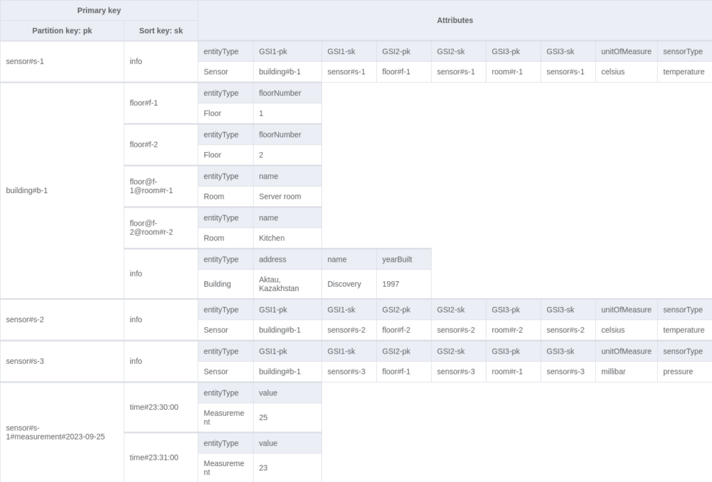
First, we create our table with a composite primary key: pk (partition key) and sk (sort or range key). Generic names are used since those fields will contain different entities. It is a good practice to put a prefix before IDs in pk and sk for readability and efficiency. The table will mainly use entity type as the prefix (building, floor, sensor, etc.).
Get building info
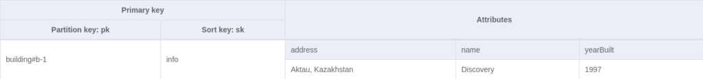
Let’s start with a simple query. The pk field contains the building ID with the prefix: `building#b-1`, whereas the sk field contains the constant value: `info`. Some developers may prefer duplicating the pk value in the sk field instead of `info`. All in all, you may get the following:
To retrieve this item, you can use the `GetItem` operation:
| Access pattern | Base table / GSI / LSI | Operation | Partition key value | Sort key value | Other conditions / filters |
| Get building info | Base table | GetItem | pk=`buildingId` | sk=`info` |
Get the building’s floor info and Get the floor’s room info
For these access patterns, we can effectively utilise our sk. Chaining multiple entity IDs in sk helps achieve the one-to-many relationship:
| pk | sk |
| parent#id | child#id#grandchild#id#greatgrandchild#id… |
Following the same pattern, we can put our building ID in the pk field and floor and room IDs in the sk field:
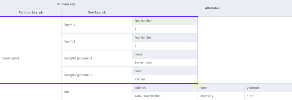
You might ask why I used `@` as a delimiter for room entities. The reason is to avoid filter expressions in query operations. However, this is a 100% overkill solution in this case because practically one building does not have so many floors and rooms to affect performance negatively. Nonetheless, if you cannot afford filter expressions, you can use that workaround, especially for deeply nested entities.
This is how you can achieve the access patterns:
| Access pattern | Base table / GSI / LSI | Operation | Partition key value | Sort key value | Other conditions / filters |
| Get the building’s floor info | Base table | Query | pk=`buildingId` | sk begins_with `floor#` | |
| Get the floor’s room info | Base table | Query | pk=`buildingId` | sk begins_with `floor@{{floorId}}@room#` |
Get the building’s sensor info, Get the floor’s sensor info and Get the room’s sensor info
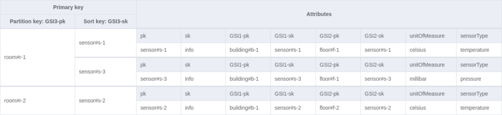
First of all, we need to decide how to store sensor information in the table. We can either continue our entity chaining in sk or put sensors under their own pk, which I did:

It would be completely fine to use the first proposed approach with the entity chaining. However, if local secondary indexes were used, and items via that approach resided under the same partition (identical partition key), it would imply the following limits:
- A single partition cannot handle more than 3000 read operations or more than 1000 write operations.
- The cumulative item size in one partition with one or more LSIs cannot exceed 10 GB. More information can be found here.
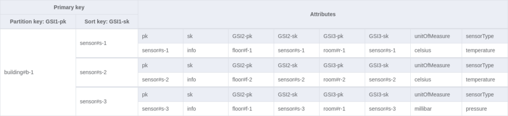
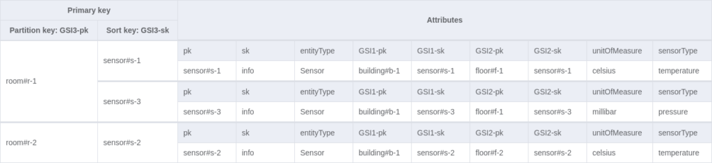
To address the access patterns, global indexes can be created. Again, we will use generic names if other entities might want to use the indexes (`GSI1-pk`, `GSI1-sk`, etc.).
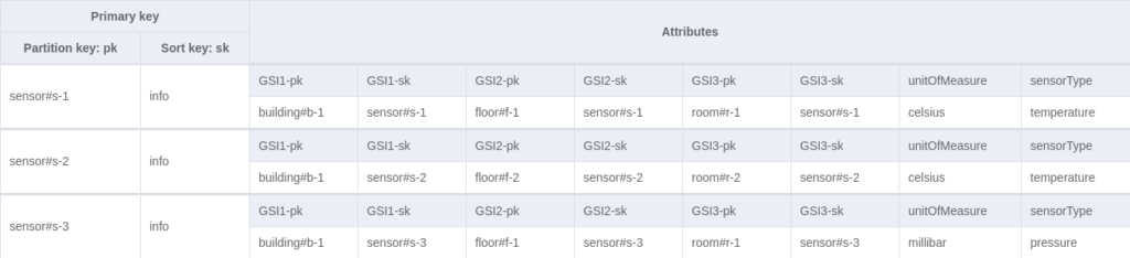
After creating all those attributes, we can create 3 GSI indexes. Note that if your table is already created, you cannot add or remove multiple indexes simultaneously.
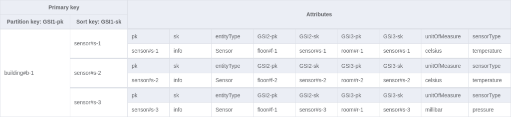

3 indexes are created, and, for simplicity, I projected all attributes in the indexes, but you may want to think twice about doing so in production. Using indexes that are utilised by all items with all projected attributes can double your storage and write operation costs. Fortunately, those indexes affect only our sensor items for now. In other words, they are sparse indexes. Also, note that when using GSIs you cannot issue transactions because they are eventually consistent.
As for operations:
| Access pattern | Base table / GSI / LSI | Operation | Partition key value | Sort key value | Other conditions / filters |
| Get the building’s sensor info | GSI 1 | Query | GSI1-pk=`buildingId` | ||
| Get the floor’s sensor info | GSI 2 | Query | GSI2-pk=`floorId` | ||
| Get the room’s sensor info | GSI 3 | Query | GSI3-pk=`roomId` |
Get the latest measurement of a particular sensor
Given the requirements, there are still many ways to place sensor measurements inside the table. My choice was to use the sensor ID and measurement date in pk and measurement time in sk:
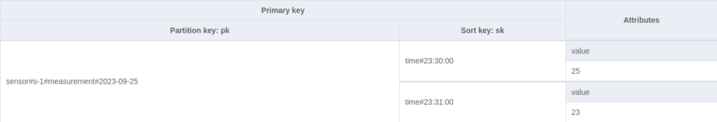
Using that structure, we can easily achieve the required access pattern, but understand that it is not the best solution for other cases. For example, we wouldn’t be able to get all measurements of a specific sensor for two or more days via one query operation. Since it is still fine for our pattern, I will leave that structure.
The latest measurement can be obtained by sorting in descending order and limiting results:
| Access pattern | Base table / GSI / LSI | Operation | Partition key value | Sort key value | Other conditions / filters |
| Get the latest measurement of a particular sensor | Base table | Query | pk=`sensorId` + current date | Limit=1ScanIndexForward=false |
Get all items of a particular entity
You might want to get data for all buildings, all rooms or all sensors. To achieve that, we can add the `entityType` field to every item and create the fourth global index. In this case, the index will consist of a partition key only.

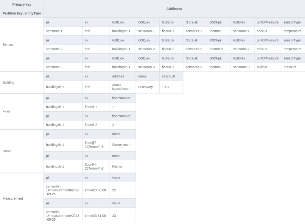
Note that this index is not sparse, so it should be cautiously implemented.
| Access pattern | Base table / GSI / LSI | Operation | Partition key value | Sort key value | Other conditions / filters |
| Get all items of a particular entity | GSI 4 | Query | entityType=`Sensor` | `Floor` | `Building` … |
Final result
We have covered a lot of techniques and access patterns. There are other uncovered topics which may further extend your design skills:
Let’s see what we have in the end:
| Access pattern | Base table / GSI / LSI | Operation | Partition key value | Sort key value | Other conditions / filters |
| Get building info | Base table | GetItem | pk=`buildingId` | sk=`info` | |
| Get the building’s floor info | Base table | Query | pk=`buildingId` | sk begins_with `floor#` | |
| Get the floor’s room info | Base table | Query | pk=`buildingId` | sk begins_with `floor@{{floorId}} @room#` | |
| Get the building’s sensor info | GSI 1 | Query | GSI1-pk=`buildingId` | ||
| Get the floor’s sensor info | GSI 2 | Query | GSI2-pk=`floorId` | ||
| Get the room’s sensor info | GSI 3 | Query | GSI3-pk=`roomId` | ||
| Get the latest measurement of a particular sensor | Base table | Query | pk=`sensorId` + current date | Limit=1 ScanIndexForward=false | |
| Get all items of a particular entity | GSI 4 | Query | entityType=`Sensor` | `Floor` | `Building` … |
New requirements do not fit!
In software development, client requirements are often subject to change. You may finish your “perfect” table design only to find out after some time that it cannot be extended because of the new requirements. There are some workarounds you can implement like creating an additional table or GSI to cater to client’s needs. However, there is a chance that you must migrate your table(s) to new ones with another schema/model. This also imposes a challenge when you cannot afford any downtime on production. Fortunately, AWS offers multiple ways for transferring your data reliably. For more information, you can refer to this post.
Conclusion
DynamoDB single-table design is substantially different from conventional SQL table modelling. There are different techniques which help implement relationships between entities in one table. We have learned how we can change and evolve our design depending on the provided access patterns. Remember that there are almost always multiple solutions to one problem. Do not stop on one design only and try experimenting more to achieve a reasonable and flexible model, but do not attempt to get a design which satisfies all possible future requirements.
Other useful sources of information:
- AWS DDB Developer guide
- More DDB modelling examples
- DDB best practices
- Single-table vs. multi-table design in DDB
By Ruslan Yeleussinov, Software Developer at Klika Tech, Inc.