Comparing Query Languages for AWS Neptune: SPARQL, Gremlin, and OpenCypher

General overview and introduction

Graph databases have gained significant traction in recent years, owing to their unique ability to model and query highly interconnected data. Among the leading providers in this space, Amazon Web Services Neptune stands out as a managed graph database service that caters to a wide range of user requirements. What makes AWS Neptune particularly compelling is its support for multiple query languages, each designed to address specific data modeling and querying needs. In this article, we will explore three of the most prominent query languages available on AWS Neptune: SPARQL, Gremlin, and OpenCypher.

The Popularity of Graph Databases

Before we delve into the nuances of these query languages, let’s take a moment to understand the growing popularity of graph databases. Traditional relational databases excel at handling structured data, but they often fall short when it comes to representing complex relationships and connections. This is where graph databases come into play. They are purpose-built to manage data that can be visualized as interconnected nodes and edges. This flexibility has made them a cornerstone of modern applications, from social networks to recommendation engines.

Overall use cases for graph databases

Graph databases are used in a wide range of different scenarios and applications.
Their ability to traverse complex relationships with ease makes them an ideal choice for scenarios involving:

1. Recommendation Engines: Graph databases excel at modeling user preferences and item relationships, making them vital for building recommendation systems that power e-commerce platforms and content streaming services.
2. Social Networks: In the world of social media, connections between users, their interests, and interactions are inherently graph-like. Graph databases can efficiently store and retrieve this data, facilitating real-time updates and personalized content delivery.
3. Fraud Detection: Detecting fraudulent activities often involves spotting intricate patterns and connections among seemingly unrelated events. Graph databases can quickly identify such anomalies by analyzing the relationships between data points.
4. Knowledge Graphs: Organizations use graph databases to build knowledge graphs that connect various pieces of information, enabling advanced semantic search and data integration.

Available query languages on AWS Neptune

Offering support for multiple query languages, AWS Neptune allows users to adapt to various data modeling and querying needs. In this section, we will explore three key query languages available on AWS Neptune: SPARQL, Gremlin, and OpenCypher. Understanding the features, advantages, and use cases of each language will enable you to make an informed decision about which one suits your specific requirements.

SPARQL (for RDF Graphs) 

• Standardized Language: SPARQL is a W3C-recommended query language tailored for RDF (Resource Description Framework) graphs. 
• Triple Patterns: Queries use triple patterns, consisting of subject (node) – predicate (edge) – object (node): ?s ?p ?o, e.g.:

?person ex:likes ?book 

• Rich Querying Capabilities: Supports filtering, aggregation, and sub-queries. 
• Advantages: Interoperability, Semantic Web focus, and support for federated queries.
• Use Cases: Ideal for knowledge graphs, linked data, and ontology management.
• Maintainer: Developed by the World Wide Web Consortium (W3C).

Gremlin (for Property Graphs)

• Graph Traversal Language: Gremlin simplifies navigation of complex graph structures.
• Imperative Style: Traversals are defined step by step.
• Extensible: Gremlin can be extended with user-defined steps.
• Advantages: Flexibility, wide adoption across graph databases, and a rich ecosystem.
• Use Cases: Suitable for social networks, recommendation engines, and fraud detection.
• Maintainer: Maintained by the Apache Software Foundation.

OpenCypher (for Property Graphs)

• Declarative Language: OpenCypher takes an SQL-like, declarative approach.
• Pattern Matching: Expresses graph shapes with ASCII-art style patterns, that so-called motif syntax, like: ()-[]->(), e.g.:

(Alice)-[:IS_FRIENDS_WITH]->(Bob)

• Rich Querying Capabilities: Supports filtering, aggregation, and ordering.
• Advantages: Intuitive syntax, expressiveness, and growing adoption.
• Use Cases: Suitable for business analytics, knowledge graphs, and network analysis.
• Maintainer: Initiated by Neo4j, promoting compatibility and portability across various graph database systems.

Before We Dive into Real-Life Projects

When planning your graph database projects on AWS Neptune, before you embark on your graph database journey with AWS Neptune, it’s crucial to understand how data loading, querying languages, and data storage are interconnected.

Data Loading and Querying Languages:

When working with AWS Neptune, your choice of data loading and querying languages has a direct impact on your project’s flexibility and capabilities:

• Gremlin and OpenCypher: If you’ve loaded your data into AWS Neptune using Gremlin or OpenCypher, you have the flexibility to query it using either Gremlin or OpenCypher. Both of these query languages are tailored to work seamlessly with property graphs, which align with the structure of your data in Neptune.
• SPARQL: To the contrary, if you’ve loaded RDF (Resource Description Framework) data into Neptune using SPARQL, your querying options are more limited. In this case, you can only query your data using SPARQL. This constraint arises because RDF datasets have a specific nature that differs from property graphs, making other query languages like Gremlin or OpenCypher unsuitable for RDF data in Neptune.
  

Data Storage in AWS Neptune:

The way data is stored in AWS Neptune is inseparably tied to the nature of the data and the query language used for data loading. Neptune optimizes its data storage format to facilitate efficient querying and traversal:

• Property Graph Data: When you load property graph data using Gremlin or OpenCypher, Neptune stores it in a way that optimally supports the property graph model. This storage format allows for efficient querying and traversal of complex graph structures.
• RDF Data: In the case of RDF data loaded using SPARQL, Neptune stores it according to the RDF data model. RDF data is typically stored as subject-predicate-object triples, enabling semantic querying and exploration of linked data.
  

To further clarify how data loading and querying languages align, here’s a simplified representation in table format:

Data loaded with	Can be queried using
Gremlin	Gremlin, openCypher
openCypher	Gremlin, openCypher
SPARQL (RDF data)	SPARQL only

In the following sections, we will explore real-life use cases and delve into the capabilities and strengths of each query language, helping you make informed decisions for your projects.

Real-life project example – our dataset and queries

Let’s begin by providing an overview of the dataset. In this article, we’ll be working with a straightforward dataset comprising two categories of nodes: Person and Book.
Additionally, it involves two kinds of relationships: likes and is friends with.

A tabular representation of the above-mentioned dataset:

Table 1: People

Name	Age
Alice	25
Bob	30
Charlie	27

Table 2: Books

Title	Genre
Graph Theory	Math
Elegant Graphs	Design
World History	History

Table 3: Relationships

Person	Relationship	Book/Person
Alice	Is friends with	Bob
Bob	Is friends with	Charlie
Alice	Likes	Graph Theory
Bob	Likes	World History
Charlie	Likes	Elegant Graphs
Charlie	Likes	Graph Theory

Queries we’re going to run:

• Query 1: Find all distinct book titles that are liked by friends of Alice.
• Query 2: Calculate the average age of individuals who like books with the genre Math.
• Query 3: Find the names of individuals who like books, exclude those who are friends with Alice, and Alice herself. Also, count the number of distinct books each person likes. Then, sort them in descending order by the number of books liked.

Sidenote: For each query, we’re going to use SageMaker Notebooks.

Example Property Graph from Neo4j Bloom

Although in this article we’re discussing AWS Neptune, I have decided to use a different tool for visualization here – Neo4j Bloom, which is a really powerful tool for visualizing property graphs. More on visualization in AWS Neptune in the last section of this article – Visualization of data in AWS Neptune Workbench.

Here’s an example of how the dataset might look in a Neo4j Bloom:

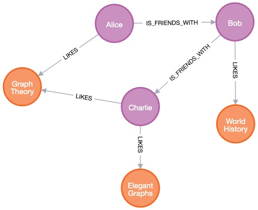
In this visualization, you can see nodes representing people and books, and relationships portraying connections such as friendships and likes. This graphical representation provides an intuitive way to explore and analyze the data in a property graph.

Next, we will proceed to demonstrate the execution of the three queries in SPARQL, Gremlin, and OpenCypher to showcase the versatility of these query languages in AWS Neptune.

We will focus mostly on the first query to show the syntax and features of each query language.
Please keep in mind that those are only example queries, the same results we can get by utilizing different queries. 

Inserting data

1. To load SPARQL data we used the following queries:

%%sparql 
PREFIX ex: <http://example.org/>
PREFIX rdf: <http://www.w3.org/1999/02/22-rdf-syntax-ns#>
    
INSERT DATA {
    GRAPH <http://example.org/graph> {
        # create Person nodes
        ex:Alice rdf:type ex:Person ;
        ex:name "Alice" ;
        ex:age 25 .
        ex:Bob rdf:type ex:Person ;
        ex:name "Bob" ;
        ex:age 30 .
        ex:Charlie rdf:type ex:Person ;
        ex:name "Charlie" ;
        ex:age 27 .
        # create Book nodes
        ex:GraphTheory rdf:type ex:Book ;
        ex:title "Graph Theory" ;
        ex:genre "Math" .
        ex:ElegantGraphs rdf:type ex:Book ;
        ex:title "Elegant Graphs" ;
        ex:genre "Design" .
        ex:WorldHistory rdf:type ex:Book ;
        ex:title "World History" ;
        ex:genre "History" .
        # Create relationships
        ex:Alice ex:isFriendsWith ex:Bob .
        ex:Bob ex:isFriendsWith ex:Charlie .
        ex:Alice ex:likes ex:GraphTheory .
        ex:Bob ex:likes ex:WorldHistory .
        ex:Charlie ex:likes ex:ElegantGraphs, ex:GraphTheory .
    }
}

2. To load Gremlin data we used the following queries:

%%gremlin
// Create Person vertices
g.addV('Person')
    .property('id', 'Alice').property('name', 'Alice').property('age', 25).next()
g.addV('Person')
    .property('id', 'Bob').property('name', 'Bob').property('age', 30).next()
g.addV('Person')
    .property('id', 'Charlie').property('name', 'Charlie').property('age', 27).next()
// Create Book vertices
g.addV('Book')
    .property('id', 'GraphTheory').property('title', 'Graph Theory').property('genre', 'Math').next()
g.addV('Book')
    .property('id', 'ElegantGraphs').property('title', 'Elegant Graphs').property('genre', 'Design').next()
g.addV('Book')
    .property('id', 'WorldHistory').property('title', 'World History').property('genre', 'History').next()
// Create relationships (edges)
g.V().has('id', 'Alice').addE('isFriendsWith').to(__.V().has('id', 'Bob')).next()
g.V().has('id', 'Bob').addE('isFriendsWith').to(__.V().has('id', 'Charlie')).next()
g.V().has('id', 'Alice').addE('likes').to(__.V().has('id', 'GraphTheory')).next()
g.V().has('id', 'Bob').addE('likes').to(__.V().has('id', 'WorldHistory')).next()
g.V().has('id', 'Charlie').addE('likes').to(__.V().has('id', 'ElegantGraphs')).next()
g.V().has('id', 'Charlie').addE('likes').to(__.V().has('id', 'GraphTheory')).next()

3. To load OpenCypher data we used the following queries:

%%opencypher
// Create Person nodes
CREATE (Alice:Person {name: "Alice", age: 25})
CREATE (Bob:Person {name: "Bob", age: 30})
CREATE (Charlie:Person {name: "Charlie", age: 27})
// Create Book nodes
CREATE (GraphTheory:Book {title: "Graph Theory", genre: "Math"})
CREATE (ElegantGraphs:Book {title: "Elegant Graphs", genre: "Design"})
CREATE (WorldHistory:Book {title: "World History", genre: "History"})
// Create relationships
CREATE (Alice)-[:IS_FRIENDS_WITH]->(Bob)
CREATE (Bob)-[:IS_FRIENDS_WITH]->(Charlie)
CREATE (Alice)-[:LIKES]->(GraphTheory)
CREATE (Bob)-[:LIKES]->(WorldHistory)
CREATE (Charlie)-[:LIKES]->(ElegantGraphs)
CREATE (Charlie)-[:LIKES]->(GraphTheory)

Real-life project: Running queries

Query 1

Find all distinct book titles that are liked by friends of Alice.

SPARQL:

%%sparql
PREFIX ex: <http://example.org/>
PREFIX rdf: <http://www.w3.org/1999/02/22-rdf-syntax-ns#>
SELECT DISTINCT ?bookTitle
WHERE {
    ?alice ex:name "Alice" ;
           ex:isFriendsWith ?friend .
    ?friend ex:likes ?book .
    ?book ex:title ?bookTitle .
}

In this query we start by defining prefixes for concise representation.
We select distinct values for the variable ?bookTitle, which we want to retrieve as results.
We use triple patterns to traverse the graph: we start with a subject identified as ?alice, who has the name Alice.
We find ?friend entities who are friends with ?alice via the ex:isFriendsWith relationship. For each ?friend, we identify ?book entities they like via the ex:likes relationship.
We extract the titles of these ?book entities as ?bookTitle.
The results are filtered based on the conditions specified in the WHERE clause.

Gremlin:

%%gremlin
g.V()
     .has('name', 'Alice')                 
     .out('isFriendsWith')                 
     .out('likes')                         
     .values('title')                      
     .dedup()

In this query, we’re navigating a graph, which consists of vertices (nodes) and edges (relationships).
We start at a vertex with the name property Alice, then traverse outgoing isFriendsWith edges to find friends. 

We continue traversing outgoing likes edges to find books liked by those friends, and at the end, we extract and deduplicate the title property from these books.

OpenCypher:

%%opencypher
MATCH (alice:Person {name: "Alice"})-[:IS_FRIENDS_WITH]->(friend:Person)-[:LIKES]->(book:Book)
RETURN DISTINCT book.title AS bookTitle

In this query, we use a SQL-like syntax to: match a vertex labeled as Person with the name property Alice, then traverse outgoing :IS_FRIENDS_WITH relationships to find friends (also Person vertices). We continue traversing outgoing :LIKES relationships to find books liked by those friends, and finally return distinct book titles as bookTitle.
OpenCypher’s SQL-like syntax and the graphic representation of relationships make it expressive and easy to read, especially for those familiar with SQL and graph databases.

Results of this query:

Query 2

Calculate the average age of individuals who like books with the genre Math.

SPARQL:

%%sparql
PREFIX ex: <http://example.org/>
PREFIX rdf: <http://www.w3.org/1999/02/22-rdf-syntax-ns#>
SELECT (AVG(?age) as ?averageAge)
WHERE {
    ?person ex:age ?age ;
            ex:likes ?book .
    ?book ex:genre "Math" .
}

Gremlin:

%%gremlin
g.V()
     .hasLabel('Book')
     .has('genre', 'Math')       
     .in('likes')                                  
     .values('age')                                
     .mean()

Opencypher:

%%opencypher
MATCH (person:Person)-[:LIKES]->(book:Book)
WHERE book.genre = "Math"
WITH AVG(person.age) AS averageAge
RETURN averageAge

Results of this query:

Query 3

Find the names of individuals who like books, exclude those who are friends with Alice, and Alice herself. Also, count the number of distinct books each person likes. Then, sort them in descending order by the number of books liked.

SPARQL:

%%sparql
PREFIX ex: <http://example.org/>
PREFIX rdf: <http://www.w3.org/1999/02/22-rdf-syntax-ns#>
SELECT ?personName (COUNT(DISTINCT ?book) AS ?numberOfBooksLiked)
WHERE {
    ?person ex:likes ?book .
    ?person ex:name ?personName .
    
    FILTER NOT EXISTS {
        ?alice ex:name "Alice" ;
               ex:isFriendsWith ?person .
    }
    
    MINUS {
        ex:Alice ex:name ?personName .
    }
}
GROUP BY ?personName
ORDER BY DESC(?numberOfBooksLiked)

Gremlin:

%%gremlin
g.V()
  .hasLabel('Person')
  .where(__.not(has('name', 'Alice')))
  .where(__.not(inE('isFriendsWith').outV().has('name', 'Alice')))
  .project('personName', 'numberOfBooksLiked')
  .by('name')
  .by(out('likes')
  .dedup()
  .count())

Opencypher:

%%opencypher
MATCH (alice:Person {name: "Alice"})
MATCH (person:Person)-[:LIKES]->(book:Book)
WHERE NOT EXISTS((alice)-[:IS_FRIENDS_WITH]-(person)) AND person <> alice
WITH person, COLLECT(DISTINCT book) AS likedBooks
RETURN DISTINCT person.name AS personName, SIZE(likedBooks) AS numberOfBooksLiked
ORDER BY numberOfBooksLiked DESC

Results of this query:

Visualization of data

Prior to summarizing, let’s take a moment to explore visualization with AWS Neptune and the AWS Neptune Workbench. AWS offers various visualization options tailored to each query language, leveraging their respective features to display data effectively.

SPARQL:

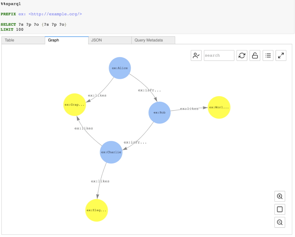
Visualizing SPARQL query results is very limited and possible only if the SPARQL query takes either one of these forms:

SELECT ?subject ?predicate ?object

SELECT ?s ?p ?o

Additionally, we have a possibility to include such literal values as vertices in the visualization. To do that, use the –expand-all query hint after the %%sparql cell magic:

%%sparql –expand-all

A simple example can be shown below:

Gremlin:

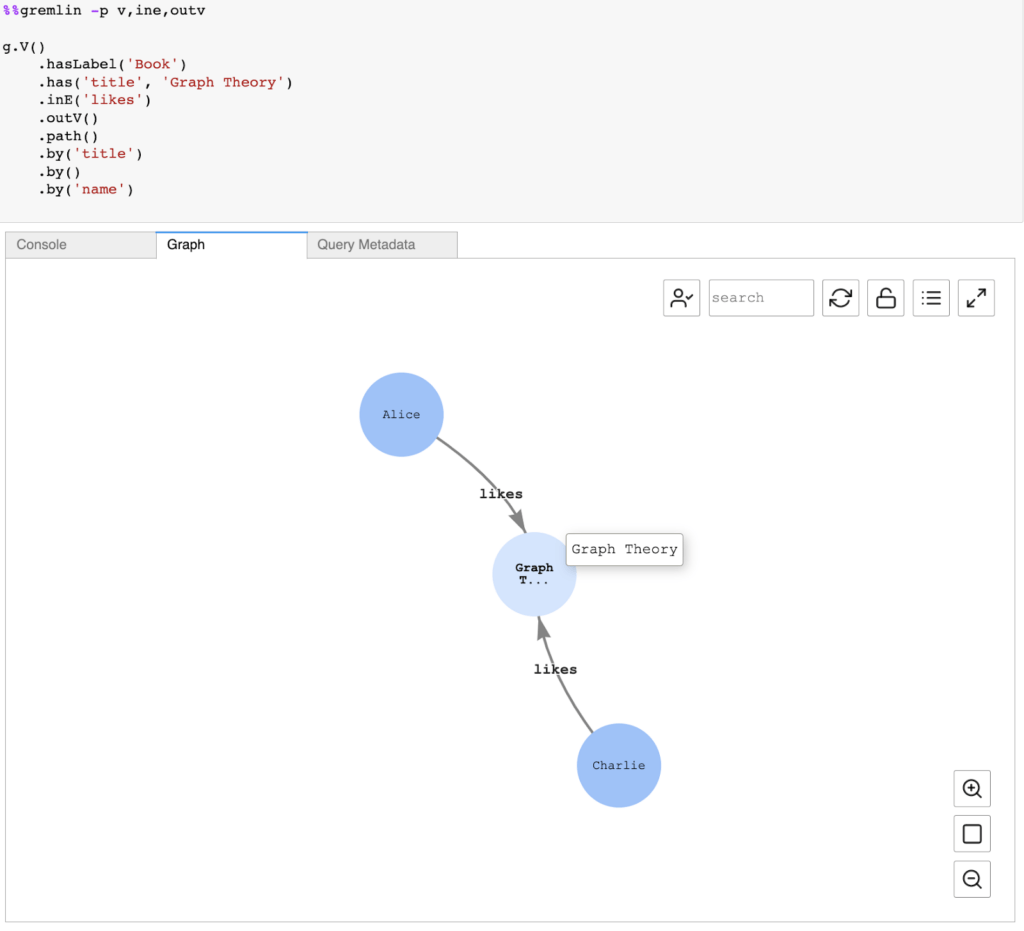
Gremlin undoubtedly offers the most extensive capabilities for presenting data among the three query languages we’ve discussed. Let’s briefly dive into the possible options here.

To control how the visualizer diagrams query output, we need to use query visualization hints. Those hints have to be added to the %%gremlin magic cell and are preceded by the –path-pattern (or its short form: -p) parameter name:

%%gremlin -p comma-separated hints

You can also use the –group-by (or -g) option to specify a property of the vertices that you want to group together. The names of the hints are based on common Gremlin steps used for moving between vertices, and they work in a way that matches these steps.
You can use multiple hints together, separated by commas (without spaces), as long as they match the Gremlin steps used in your query. Here is an example showing all people who like the book Graph Theory with relationships and its direction:

OpenCypher:

When it comes to the visualization of data, OpenCypher has also quite limited functionality. ​​
You can visualize the outcomes of any openCypher query that yields a path:

MATCH p= … RETURN p

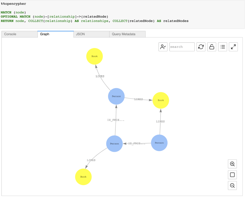
or a basic list of nodes in a graphical format. You can specify query visualization hints using -d, -de, -l, and -g after the %%oc or %%opencypher magic cell. Either one of them can be used to run an openCypher query, for more details please refer to the table presented below.

Query visualization hint	Stands for
-d	vertex mapping
-de	edge mapping
-l	max label length
-g	property to group by

For Opencypher, we can also use any tool that is able to visualize property graphs, not necessarily stored in Gremlin format (vertex and edge files). 

Changing the visualization settings

Neptune notebooks utilize an open-source tool called Vis.js for creating graphical representations of graphs.
If you want to check the current settings being used in your notebook, you can run the %graph_notebook_vis_options command, and you will get a JSON-based list with all current settings.
To adjust any of these settings, follow these steps: create a new cell, copy the existing settings, make the desired changes, and then apply %%graph_notebook_vis_options (note the double percent signs indicating a cell-level command) to put the modifications into effect.

Conclusion

The choice between SPARQL, Gremlin, and OpenCypher largely depends on the nature of your data and the specific use case. If you’re working with RDF graphs and linked data, SPARQL is the go-to choice. For property graphs, both Gremlin and OpenCypher have their merits. Gremlin’s traversal-centric approach is powerful for complex navigations, while OpenCypher’s declarative style is more intuitive for those familiar with SQL-like languages.

Regardless of the choice, AWS Neptune’s support for multiple query languages ensures that users have the flexibility to choose the best tool for their specific needs.

By Grzegorz Wawrzak, Senior Software Developer at Klika Tech, Inc.